
The constraint is connectivity, not just bandwidth.
A high-bandwidth module is useful only if its capacity reaches the peers the topology needs. Treat an entire module as one indivisible connection and its lanes all terminate on the same neighbor. Configure supported breakout modes and those lanes can instead form several independent links. The switch still has the same aggregate bandwidth, but it can address more neighbors.
At AI-cluster scale, this becomes an architectural decision. More usable ports at a narrower link width can let a two-tier leaf–spine network reach more endpoints before another switching tier is required. The optical shuffle packages the resulting connectivity matrix into repeatable fiber assemblies. It is the physical implementation of the topology, with every source lane assigned to a destination. IEEE E4AI architecture discussion
Read the fabric in two dimensions: rails and planes.
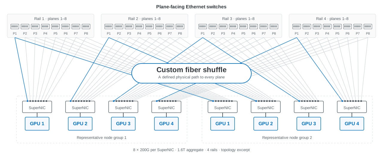
In the opening diagram, a rail groups corresponding GPU/SuperNIC positions across the node groups. A plane provides an independent network path carrying part of each NIC’s bandwidth. The four rail groups across the top each expose eight plane-facing connections; every depicted SuperNIC reaches all eight planes in its own rail. The shuffle sits between the node-facing and plane-facing connector groupings.
NVIDIA describes an 800G ConnectX interface divided across four 200G planes, with passive shuffle boxes or trunks connecting the host to those networks. The NIC distributes traffic and responds to plane congestion; the fibers provide fixed paths. The opening eight-plane illustration and this four-plane example describe different configurations. NVIDIA multiplane architecture
Rails and planes must remain separate fields in the connection schedule. Two links with the right rate but the wrong rail or plane assignment can satisfy a continuity check and still implement the wrong network.
Why a flatter fabric can change the economics.
For endpoints on different leaves, a two-tier path crosses leaf → spine → leaf. A three-tier path crossing pods can traverse leaf → aggregation → core → aggregation → leaf. Where supported breakout and plane connectivity allow the required endpoint population to remain in two tiers, the design avoids those additional switching stages and their associated interconnects. Architecture comparison
Compare complete designs at the same endpoint count, aggregate endpoint bandwidth and failure requirements. Include switches, physical transceiver modules, optical links, shuffle assemblies, patching, installation labor, spare capacity and power. A percentage taken from another topology is not a bill of materials. An added shuffle connector also consumes optical budget, and a shared enclosure can concentrate maintenance exposure.
Worked example: preserve bandwidth and count every switch.
This is an idealized calculation using a 51.2T switch with 64 × 800G or 256 × 200G usable logical interfaces. Assume supported four-way breakout at both ends, one 800G scale-out NIC per endpoint, equal downlink/uplink bandwidth, no oversubscription, no reserved ports and one leaf–spine link per pair. These are topology assumptions, not a deployment recommendation. Documented switch modes
| Quantity | 800G links / one plane | 200G links / four planes |
|---|---|---|
| Logical radix per switch | 64 | 256 |
| Host-facing links per leaf | 32 | 128 per plane |
| Leaf / spine switches | 64 / 32 | 256 / 128 per plane |
| Distinct endpoints | 2,048 | 32,768, present in all four planes |
| Bandwidth per endpoint | 800G | 4 × 200G = 800G |
| Total switches | 96 | 1,536 |
The endpoint ceiling follows the ideal two-tier expression N = radix² / 2: 64 × 32 = 2,048 versus 256 × 128 = 32,768. In the four-plane case, each leaf carries 128 × 200G = 25.6T down and 25.6T up; each spine terminates 256 × 200G = 51.2T.
Across four planes there are 131,072 host-facing 200G circuits and 131,072 leaf–spine circuits. There are still 32,768 distinct endpoints, each with four connections. Both endpoint capacity and switch inventory rise 16-fold. The gain is a larger connected network at the same tier depth—not extra bandwidth from an unchanged set of switches. Actual systems also need reserved capacity, failure modeling and a verified distribution of traffic.
What the shuffle actually changes.
A simple 4×4 permutation takes four parallel interfaces and redistributes one bidirectional lane from each into each output bundle. If A, B, C and D identify the inputs, the outputs become:
| Output bundle | Lane circuits |
|---|---|
| 1 | A1 · B1 · C1 · D1 |
| 2 | A2 · B2 · C2 · D2 |
| 3 | A3 · B3 · C3 · D3 |
| 4 | A4 · B4 · C4 · D4 |
That is 16 duplex circuits using 32 fibers, with four eight-fiber connector interfaces on each side. Each circuit retains its own transmitter and receiver path. The diagram is a logical permutation; cavity positions, key orientation, gender and Tx/Rx polarity belong in the manufacturing map. Corning documents 2×2, 4×4 and 8×8 arrangements. Corning shuffle reference
The group size follows the actual optical interface. A 200G link carried over two 100G optical lanes needs both lanes kept together; an exposed 200G optical lane has different fiber accounting. A wavelength-multiplexed FR4 duplex connection does not expose four separate fiber pairs for an ordinary passive lane shuffle. Specify the optical PMD as well as the electrical breakout mode. NVIDIA parallel and WDM interfaces
Harness, cassette or box: choose the service boundary.
| Construction | Useful when | Engineering tradeoff |
|---|---|---|
| Shuffle harness or trunk | Endpoints and routes are stable; the matrix can be factory wired into the assembly. | Custom leg lengths and routing simplify installation; replacement affects the connected bundle. |
| Modular cassette | The installation benefits from standard patching and replaceable mapping units. | Connector access and incremental replacement improve serviceability; extra mating points consume loss budget. |
| Rack-mounted shuffle box | A large repeated matrix needs a defined location, labeling and cable-management boundary. | Allocate rack space, routing clearances and replacement scope; physical co-location can create shared exposure. |
AFL describes these as alternative ways to package meshing, including custom trunks and modular assemblies. The selection should follow how the installation will be built, changed and repaired. AFL meshing whitepaper
Internal fiber optic flex circuits can implement complex permutations inside an enclosure. Molex documents custom 1–6 RU shuffle boxes spanning 72–6,400 fibers. Those are examples of manufacturing scale, not dimensions or capacities promised for a WBN design. Embedded optical-engine shuffles and external rack cabling share mapping principles but have different mechanical and service requirements. Molex construction reference
From topology to a buildable cable plant.
WBN engineers custom shuffle boxes and cabling around the required fabric. The design starts with a connection matrix and ends with an assembly that installers can identify, route and verify.
- Logical topology: endpoint, GPU position, rail, plane, switch port, link rate and failure domain.
- Platform allocation: cage, subport, lane group, FEC/application mode and firmware support. Document any adjacent-port restrictions.
- Optical continuity: source Tx to destination Rx for every used fiber, connector cavity, polish, pinning and key orientation; account separately for unused positions.
- Mechanical construction: trunk length, staggered or individual legs, bend limits, strain relief, access and removable-unit boundaries.
- Loss and identification: budget every mating interface and fiber segment, assign durable endpoint labels, and retain per-path continuity and loss records.
Release the topology and cable drawings together. Keep logical links, physical modules, occupied connector positions and cable assemblies as separate quantities so procurement and installation describe the same network.
Validate the installed fabric at three levels.
First prove the physical matrix: every intended path, polarity and loss result. Then prove each configured link: module/application recognition, negotiated mode, per-lane errors and FEC behavior under load. Finally exercise the fabric: collective traffic, incast, mixed traffic, link failures and maintenance scenarios.
A correct fiber permutation cannot compensate for unsupported NIC plane operation or an unsuitable routing and congestion policy. Conversely, a successful benchmark on one path does not establish correct wiring across every plane. Keep both the assembly records and the workload evidence attached to the deployed revision.
Sources and applicability
Original WBN engineering reference, checked 2 November 2026. The opening figure is a conceptual redraw of a published NVIDIA architecture; the four-plane calculation below is an explicitly separate example. Neither is a WBN deployment claim. Actual topology, platform modes, optical interfaces and fiber mapping must be established for the selected hardware.
-
NVIDIA — Spectrum-X Ethernet and multiplane topology
Source of the supplied architecture figure and host-edge plane explanation; platform-specific behavior.
-
Jose M. Castro — Optical Shuffle Architectures for Large AI Networks
February 2026 E4AI technical contribution, not an IEEE normative specification. Radix is a port count, not switch inventory.
-
NVIDIA SN5000 — interfaces and cable installation
4×200G mode and adjacent-cage restrictions for other breakout arrangements. The topology calculation is WBN arithmetic under stated assumptions.
-
Corning LAN-3440-AEN — shuffling for AI/ML GPU clusters
Parallel-fiber permutations, construction choices and optical loss considerations.
-
NVIDIA LinkX — 100G PAM4 product-line overview
Parallel SR4/DR4 versus duplex WDM arrangements; use the specific module application.
-
AFL — Meshing in AI and Hyperscale Data Centers
Harness, cassette and trunk implementation tradeoffs.
-
Molex — OptoConnect Aggregation Fiber Shuffle Boxes
Examples of custom fiber routing and enclosure scale, not WBN product specifications.